# Define the output directoryoutput_dir <-here('output/field_cage_experiment/raw_visualization/')# List of plots and their corresponding file namesplots <-list("plant_nutrients_date_raw_graph"= date_raw_graph,"plant_nutrients_plot_raw_graph"= plot_raw_graph,"plant_nutrients_treatment_raw_graph"= treatment_raw_graph)# Loop through each plot and save itfor (name innames(plots)) {ggsave(filename =file.path(output_dir, paste0(name, ".png")),plot = plots[[name]],width =10, height =10, dpi =300 )}
Warning message:
“Removed 18 rows containing missing values or values outside the scale range
(`geom_point()`).”
Warning message:
“Removed 18 rows containing missing values or values outside the scale range
(`geom_point()`).”
Warning message:
“Removed 18 rows containing missing values or values outside the scale range
(`geom_point()`).”
Warning message:
“Removed 18 rows containing missing values or values outside the scale range
(`geom_point()`).”
Warning message:
“Removed 18 rows containing missing values or values outside the scale range
(`geom_point()`).”
Warning message:
“Removed 18 rows containing missing values or values outside the scale range
(`geom_point()`).”
Warning message:
“Removed 18 rows containing missing values or values outside the scale range
(`geom_point()`).”
Warning message:
“Removed 18 rows containing missing values or values outside the scale range
(`geom_point()`).”
Warning message:
“Removed 18 rows containing missing values or values outside the scale range
(`geom_point()`).”
Warning message:
“Removed 18 rows containing missing values or values outside the scale range
(`geom_point()`).”
Modeling Overview
In this analysis, we are evaluating four Generalized Additive Models (GAMs) to understand the effects of fertilizer treatment and date on plant protein and carbohydrate content. Each model differs in the complexity of its random effects structure. Here is a summary of each model:
Model 1: Full Model with Cross and Nested Random Effects
Fixed Effects: Includes treatment and date, as well as their interaction (treatment * date).
Random Effects:
s(species, bs="re"): Random effect for different grass species.
s(plot_cage, bs="re"): Random effect for spatial positioning within plot cages.
Purpose: This model captures both the fixed effects of treatment and date, along with random variations across species and spatial positions, providing a comprehensive view of the variability in plant nutrient content.
Model 2: Removed Spatial Nested Random Effect
Fixed Effects: Same as Model 1, including treatment, date, and their interaction.
Random Effects:
s(species, bs="re"): Random effect for different grass species.
Purpose: This model simplifies the random effects structure by excluding the spatial random effect (plot_cage). It helps to assess how removing the spatial component affects the fit and interpretation of the model.
Model 3: No Random Effects of Grass Species and Spatial Positioning
Fixed Effects: Includes treatment and date, with their interaction.
Random Effects: None.
Purpose: This model serves as a baseline by including only the fixed effects and excluding all random effects. It provides a straightforward view of the impact of treatment and date on nutrient content without accounting for variability due to species or spatial positioning.
Model 4: Intercept Only Model
Fixed Effects: Only includes an intercept term.
Random Effects: None.
Purpose: This model acts as a null model or intercept-only model. It estimates the overall mean of the response variables (carb_mg_mg and protein_mg_mg) without considering any predictors. This model helps in understanding the baseline level of nutrient content.
Summary
By comparing these models, we aim to understand how different levels of model complexity (in terms of random effects) impact the fit and interpretation of our GAMs. The results from these models will help us identify the most appropriate model structure for explaining variations in plant protein and carbohydrate content
In [9]:
# model 1: full model with species, plot, and cage random effectsmod1 <-gam(list( carb_mg_mg ~ treatment * date +s(species,bs="re") +s(plot,bs="re") +s(cage,bs="re"), protein_mg_mg ~ treatment * date +s(species,bs="re") +s(plot,bs="re") +s(cage,bs="re")),family=mvn(d=2),select=TRUE, data=plant_nutrients)# model 2: full model with species and plot random effectsmod2 <-gam(list( carb_mg_mg ~ treatment * date +s(species,bs="re") +s(plot,bs="re"), protein_mg_mg ~ treatment * date +s(species,bs="re") +s(plot,bs="re")),family=mvn(d=2),select=TRUE, data=plant_nutrients)# model 3: removed spatial nested random effectmod3 <-gam(list( carb_mg_mg ~ treatment * date +s(species,bs="re"), protein_mg_mg ~ treatment * date +s(species,bs="re")),family=mvn(d=2),select=TRUE, data=plant_nutrients)# model 4: no random effects of grass species and spatial positioningmod4 <-gam(list( carb_mg_mg ~ treatment * date, protein_mg_mg ~ treatment * date),family=mvn(d=2),select=TRUE, data=plant_nutrients)# model 5: intercept only modelmod5 <-gam(list( carb_mg_mg ~1, protein_mg_mg ~1),family=mvn(d=2),select=TRUE, data=plant_nutrients)
Model Diagnostics
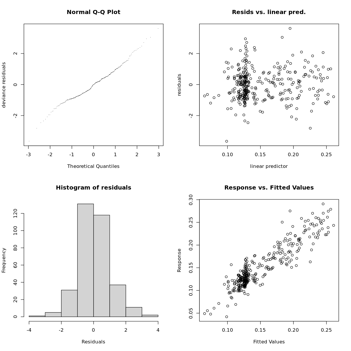
To see how well these models fit, I will run mgcv::gam.check() on it
In [10]:
gam.check(mod1)
Method: REML   Optimizer: outer newton
full convergence after 21 iterations.
Gradient range [-0.0003103183,0.0006675309]
(score -1038.257 & scale 1).
Hessian positive definite, eigenvalue range [0.04610883,3.930483].
Model rank =  127 / 127

Basis dimension (k) checking results. Low p-value (k-index<1) may
indicate that k is too low, especially if edf is close to k'.

                k'   edf k-index p-value
s(species)    7.00  4.32      NA      NA
s(plot)       9.00  1.07      NA      NA
s(cage)      37.00  2.50      NA      NA
s.1(species)  7.00  5.02      NA      NA
s.1(plot)     9.00  7.42      NA      NA
s.1(cage)    37.00 13.88      NA      NA
These diagnostic plots indicate these models are pretty well fit.
there is some discernable relationship in the variance plot, but it could be worse
Model selection criteria
In [11]:
# Model selection using AIC, BIC, and AICcbic <-BIC(mod1, mod2, mod3, mod4, mod5) |># Bayesian Information Criterionmutate(deltaBIC = BIC -min(BIC)) |>rownames_to_column('model') |> dplyr::select(model,BIC,deltaBIC)aic <-AIC(mod1, mod2, mod3, mod4, mod5) |># Akaike Information Criterionmutate(deltaAIC = AIC -min(AIC)) |>rownames_to_column('model') |> dplyr::select(model,AIC,deltaAIC)aicc <-AICc(mod1, mod2, mod3, mod4, mod5) |># AIC adjusted for small sample sizemutate(deltaAICc = AICc -min(AICc)) |>rownames_to_column('model') |> dplyr::select(model,AICc,deltaAICc)model_selection_tables <- bic |>left_join(aic,by='model') |>left_join(aicc,by='model') |>mutate(experiment ='plant_nutrients_through_time')
In [12]:
model_selection_tables |>arrange(deltaAIC)
A data.frame: 5 × 8
model
BIC
deltaBIC
AIC
deltaAIC
AICc
deltaAICc
experiment
<chr>
<dbl>
<dbl>
<dbl>
<dbl>
<dbl>
<dbl>
<chr>
mod1
-2012.394
69.42298
-2223.967
0.000000
-2130.196
54.63740
plant_nutrients_through_time
mod2
-2081.817
0.00000
-2214.475
9.491908
-2184.833
0.00000
plant_nutrients_through_time
mod3
-2059.623
22.19326
-2157.263
66.704222
-2142.409
42.42384
plant_nutrients_through_time
mod4
-2018.892
62.92436
-2084.496
139.471257
-2078.167
106.66645
plant_nutrients_through_time
mod5
-1997.612
84.20478
-2013.232
210.735098
-2012.861
171.97190
plant_nutrients_through_time
selection criteria did not agree
there were significant differences between the selection criteria. BIC and AICc selected model 2 whereas AIC selected model 1
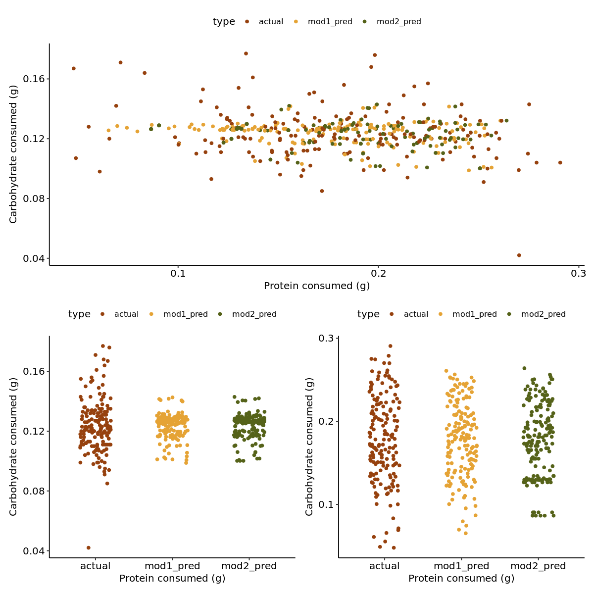
Lets view the estimates from both models to see where they agree and disagree
In [13]:
selection_testing_data <- plant_nutrients# Model 1selection_testing_data$mod1_pred_carb <-predict(mod1, newdata = plant_nutrients, type ="response")[, 1]selection_testing_data$mod1_pred_protein <-predict(mod1, newdata = plant_nutrients, type ="response")[, 2]# Model 2selection_testing_data$mod2_pred_carb <-predict(mod2, newdata = plant_nutrients, type ="response")[, 1]selection_testing_data$mod2_pred_protein <-predict(mod2, newdata = plant_nutrients, type ="response")[, 2]
In [14]:
selection_testing_data2 <- selection_testing_data |>select(carb_mg_mg, protein_mg_mg, mod1_pred_carb, mod1_pred_protein, mod2_pred_carb, mod2_pred_protein) %>%mutate(row =row_number()) |>pivot_longer(cols =starts_with("mod1_pred") |starts_with("mod2_pred") |contains("carb") |contains("protein"),names_to =c("type", "component"),names_pattern ="(.*)_(.*)$",values_to ="value" ) |>mutate(component =case_when( type =='carb_mg'~'carb', type =='protein_mg'~'protein',TRUE~ component ),type =case_when( type %in%c('carb_mg', 'protein_mg') ~'actual',TRUE~ type ) ) |>pivot_wider(names_from = component,values_from = value )
The predictions really dont change much. I think I will stick with model 1 as it better portrays the nature of the data, even if the predictions remain the same.
Plant Carbohydrate Content: The application of urea (nitrogen) as a medium treatment significantly reduced carbohydrate content compared to the control, particularly on December 1, 2015. Significant species-specific variation in carbohydrate content was observed, while plot and cage variability were not significant.
Plant Protein Content: Surprisingly, despite the urea (nitrogen) fertilization, the high treatment reduced protein levels in plants, contrary to what might be expected. Significant changes in protein content were observed on November 25 and December 1, 2015. There were notable effects from species, plot, and cage variability, with species and plot effects being particularly strong.
Overall Model Performance: The model explains 70.4% of the deviance in carbohydrate and protein content, indicating a very good fit.
Model outputs and raw data
I am going to get the estimated marginal means for treatment,date, and treatment:date and output as a dataframe
I will also write out to disk the model object
In [17]:
plant_nutrient_exp_preds <-expand.grid(species =unique(plant_nutrients$species),treatment =unique(plant_nutrients$treatment),date =unique(plant_nutrients$date),plot =unique(plant_nutrients$plot),cage =unique(plant_nutrients$cage))# Predict carbohydrate consumptionplant_nutrient_exp_preds$pred_carb <-predict(mod3, newdata = plant_nutrient_exp_preds, type ="response")[, 1]# Predict protein consumptionplant_nutrient_exp_preds$pred_protein <-predict(mod3, newdata = plant_nutrient_exp_preds, type ="response")[, 2]# Now averaging arcoss species, plot, and cageplant_nutrient_exp_preds2 <- plant_nutrient_exp_preds |>group_by(date,treatment) |>summarize(pred_carb =mean(pred_carb),pred_protein =mean(pred_protein))
`summarise()` has grouped output by 'date'. You can override using the
`.groups` argument.
In [18]:
write.csv(plant_nutrient_exp_preds2,here('data/processed/field_cage_experiment/plant_nutrient_predictions.csv'),row.names=FALSE)write.csv(plant_nutrients,here('data/processed/field_cage_experiment/plant_nutrient_raw_data.csv'),row.names=FALSE)write.csv(model_selection_tables, here("output/field_cage_experiment/plant_nutrient_model_selection_criteria_results.csv"),row.names=FALSE)# Combine the lists into a single listmodels <-list('mod1'= mod1, 'mod2'= mod2, 'mod3'= mod3, 'mod4'= mod4)# Save the combined list to an RDS filesaveRDS(models, here("output/field_cage_experiment/model_objects/plant_nutrient_through_time_models.rds"))
Section 2 - Species-specific and soil nutrient content by fertilization treatment