This script analyzes the locust data (protein and carbohydrates) for the field cage experiments

Please see manuscript for specific methodology.

This script does the following:

analyze locust weight, surivial, and # adult in field cages
analyze locust nutrient rebalancing through time

Manuscript figure preparation happens in the 03_field_cages_intake_target_mauscript_figure_code.ipynb file

In [2]:

load_packages <- function(packages) {
  # Check for uninstalled packages
  uninstalled <- packages[!packages %in% installed.packages()[,"Package"]]
  
  # Install uninstalled packages
  if(length(uninstalled)) install.packages(uninstalled, dependencies = TRUE)

  # Load all packages
  for (pkg in packages) {
    if (!require(pkg, character.only = TRUE, quietly = TRUE)) {
      message(paste("Failed to load package:", pkg))
    }
  }
}

# List of packages to check, install, and load
packages <- c("mgcv", "MuMIn", "multcomp", "gratia", 
              "ggpubr", "patchwork", "broom", "knitr", "janitor", 
              "here","ggpubr","MetBrewer","GGally","tidyverse")

load_packages(packages)

i_am('README.md')

# Functions
                   
## Standard error
std <- function(x) sd(x)/sqrt(length(x))


# Setting R options for jupyterlab
options(repr.plot.width = 10, repr.plot.height = 10,repr.matrix.max.rows=10)

here() starts at /home/datascience/herbivore_nutrient_interactions

Section 1 - analyze locust weight, surivial, and # adult in field cages

read in data

In [3]:

adult_survival_prop <- read_csv(here("data/raw/field_cage_experiment/LocustCageData_v02.xlsx - by cage.csv"),show_col_types = FALSE) 

final_mass <- read_csv(here("data/raw/field_cage_experiment/LocustCageData.csv"),show_col_types = FALSE) |>
  mutate(Treatment = fct_recode(Treatment, "None" = "0N", "Medium" = "MedH", "High" = "HighN"))

New names:
• `` -> `...24`
• `` -> `...25`
• `` -> `...26`
• `` -> `...27`
• `` -> `...28`

Now create two dataframes

survival and adult proporation at end of field cage experiment
final mass of all surviving locusts at end of experiment

In [6]:

adult_survival_prop2 <- adult_survival_prop |>
    dplyr::select(`N level`,cageNum,AdultProportion,SurviveProportion) |>
    clean_names() |>
    mutate(n_level = factor(n_level),
           treatment = fct_recode(n_level, "None" = '0', "Medium" = '87.5', "High" = '175')) |>
    select(!n_level)

In [7]:


final_mass2 <- final_mass |>
    clean_names() |>
    filter(!complete.cases(oedaleus_australis)) |>
    select(treatment,mass_g,sex)

save to disk for figure construction

In [8]:

write.csv(adult_survival_prop2, here("data/raw/field_cage_experiment/adult_locust_proportion_survival_by_treatment.csv"),row.names=FALSE)

write.csv(final_mass2, here("data/raw/field_cage_experiment/adult_locust_final_mass_by_treatment.csv"),row.names=FALSE)

Section 2 - analyze locust nutrient rebalancing through time

read in data

We need to read in the data and conduct some significant management

In [9]:


# Read and clean the names
dat <- suppressMessages(read_csv(here("data/raw/field_cage_experiment/Field_Cage_IT.csv"),
                show_col_types = FALSE, skip = 1) |>
  clean_names() |>
  as_tibble())

dat |> head()

A tibble: 6 × 53
locust_id_num	field_plot	field_cage_num	date_collected_from_field	color	sex	locust_initialmass_g	locusts_final_mass_g	notes	molt_date	⋯	high_prot_final_g_44	x45	diet_change5_start_time	diet_change5_end_time	high_carb_dish_num_48	high_carb_initial_g_49	high_carb_final_g_50	high_prot_dish_num_51	high_prot_initial_g_52	high_prot_final_g_53
<dbl>	<chr>	<dbl>	<chr>	<chr>	<chr>	<dbl>	<dbl>	<chr>	<chr>	⋯	<dbl>	<lgl>	<chr>	<chr>	<dbl>	<dbl>	<dbl>	<dbl>	<dbl>	<dbl>
101	C1	5	Nov 23, 2015 7:00 PM	B	F	0.353	0.330	NA	Nov 30, 2015	⋯	2.888	NA	Nov 29, 2015 8:00 PM	Dec 2, 2015	123	2.954	2.941	90	2.924	2.9250
102	C1	5	Nov 23, 2015 7:00 PM	B	M	0.167	0.165	NA	Dec 1, 2015	⋯	2.887	NA	NA	NA	146	2.868	2.868	85	2.856	2.8540
103	C1	6	Nov 23, 2015 7:00 PM	B	F	0.300	NA	Dead2nd day; prob no eat	NA	⋯	NA	NA	NA	NA	NA	NA	NA	NA	NA	NA
104	C1	7	Nov 23, 2015 7:00 PM	G	F	0.262	NA	Died 1 Dec	NA	⋯	2.932	NA	NA	NA	106	2.841	2.839	101	2.852	2.8532
105	H1	1	Nov 23, 2015 7:00 PM	B	F	0.156	NA	Dead2nd day; prob no eat	NA	⋯	NA	NA	NA	NA	NA	NA	NA	NA	NA	NA
106	H1	2	Nov 23, 2015 7:00 PM	B	F	0.211	0.328	NA	NA	⋯	2.905	NA	NA	NA	116	2.894	2.858	58	2.906	2.8680

data management step 1

dropping NAs
identifying treatments based on cage number
creating time series for locust IT (step 1-5)

In [11]:

dat2 <- dat |>
  drop_na(locusts_final_mass_g) |>
  mutate(
    sex = if_else(sex == 'B', 'M', sex),
    treatment = case_when(
      field_cage_num %in% c(1:4, 21:24, 29:32) ~ "High",
      field_cage_num %in% c(9:12, 17:20, 25:28) ~ "Med",
      field_cage_num %in% c(5:8, 13:16, 33:36) ~ "none"),
    total_c_step1 = (`high_carb_initial_g_14` - `high_carb_final_g_15`) * 0.42,
    total_p_step1 = (`high_prot_initial_g_17` - `high_prot_final_g_18`) * 0.42,
    total_c_step2 = (`high_carb_initial_g_22` - `high_carb_final_g_23`) * 0.42,
    total_p_step2 = (`high_prot_initial_g_25` - `high_prot_final_g_26`) * 0.42,
    total_c_step3 = (`high_carb_initial_g_31` - `high_carb_final_g_32`) * 0.42,
    total_p_step3 = (`high_prot_initial_g_34` - `high_prot_final_g_35`) * 0.42,
    total_c_step4 = (`high_carb_initial_g_40` - `high_carb_final_g_41`) * 0.42,
    total_p_step4 = (`high_prot_initial_g_43` - `high_prot_final_g_44`) * 0.42,
    total_c_step5 = (`high_carb_initial_g_49` - `high_carb_final_g_50`) * 0.42,
    total_p_step5 = (`high_prot_initial_g_52` - `high_prot_final_g_53`) * 0.42,
  )

In [12]:

dat2

A tibble: 30 × 64
locust_id_num	field_plot	field_cage_num	date_collected_from_field	color	sex	locust_initialmass_g	locusts_final_mass_g	notes	molt_date	⋯	total_c_step1	total_p_step1	total_c_step2	total_p_step2	total_c_step3	total_p_step3	total_c_step4	total_p_step4	total_c_step5	total_p_step5
<dbl>	<chr>	<dbl>	<chr>	<chr>	<chr>	<dbl>	<dbl>	<chr>	<chr>	⋯	<dbl>	<dbl>	<dbl>	<dbl>	<dbl>	<dbl>	<dbl>	<dbl>	<dbl>	<dbl>
101	C1	5	Nov 23, 2015 7:00 PM	B	F	0.353	0.330	NA	Nov 30, 2015	⋯	0.00000	0.00000	0.01848	0.00168	0.00840	0.00252	0.00042	0.00126	0.00546	-0.00042
102	C1	5	Nov 23, 2015 7:00 PM	B	M	0.167	0.165	NA	Dec 1, 2015	⋯	0.00000	0.00042	0.00756	0.00000	0.00966	0.00252	0.00000	0.00420	0.00000	0.00084
106	H1	2	Nov 23, 2015 7:00 PM	B	F	0.211	0.328	NA	NA	⋯	0.00798	0.00000	0.01050	0.00000	0.03738	0.00882	0.02478	0.01512	0.01512	0.01596
107	H1	2	Nov 23, 2015 7:00 PM	G	F	0.216	0.313	NA	NA	⋯	0.01764	0.00042	0.01512	0.00168	0.01974	0.01218	0.02226	0.01680	0.00084	0.00000
108	H1	3	Nov 23, 2015 7:00 PM	B	F	0.192	0.252	NA	NA	⋯	0.01344	0.00000	0.01008	0.00168	0.01176	0.00336	0.02016	0.00336	0.01764	0.00168
⋮	⋮	⋮	⋮	⋮	⋮	⋮	⋮	⋮	⋮	⋱	⋮	⋮	⋮	⋮	⋮	⋮	⋮	⋮	⋮	⋮
133	C3	34	Nov 23, 2015 7:00 PM	M	M	0.121	0.138	NA	NA	⋯	0.00252	0.00000	0.00420	0	0.00714	0.00168	0.00672	0.00126	0.00336	0.00420
134	C3	34	Nov 23, 2015 7:00 PM	B	F	0.293	0.213	Wing buds separating	Nov 30, 2015	⋯	0.00546	0.00000	0.00336	0	0.00252	0.00042	0.00126	0.00084	-0.83664	0.00084
136	C3	36	Nov 23, 2015 7:00 PM	B	F	0.231	0.225	NA	NA	⋯	-0.00126	0.00000	0.00000	0	0.01764	0.00168	0.00588	0.00126	0.00042	0.00042
137	H3	31	Nov 23, 2015 7:00 PM	G	F	0.215	0.336	NA	NA	⋯	0.00294	0.00042	0.00588	0	0.00714	0.00210	0.01302	0.01050	0.02142	0.01680
138	H3	32	Nov 23, 2015 7:00 PM	B	M	0.134	0.135	NA	NA	⋯	0.00126	0.00000	0.00462	0	0.00630	0.00168	0.00462	0.00252	0.00924	0.00336

data management step 2

filter consumption step for negative numbers
creating a row ID
collasping the time steps into a longer format
recoding the time step into a simple number

In [13]:


dat3 <- dat2|>
  filter(
    total_c_step1 >= 0, total_p_step1 >= 0,
    total_c_step2 >= 0, total_p_step2 >= 0,
    total_c_step3 >= 0, total_p_step3 >= 0,
    total_c_step4 >= 0, total_p_step4 >= 0,
    total_c_step5 >= 0, total_p_step5 >= 0
  ) |>
  mutate(id = row_number()) |>
  pivot_longer(cols = c(starts_with("total_c_"), starts_with("total_p_")),
               names_to = c(".value", "interval"), 
               names_pattern = "(.*)_(.*)") |> 
  select(field_plot,field_cage_num, sex,locust_initialmass_g,locusts_final_mass_g, treatment,id,interval,total_c,total_p) |>
  mutate(interval = recode(interval, 
                           step1 = "1", 
                           step2 = "2", 
                           step3 = "3", 
                           step4 = "4", 
                           step5 = "5"),
        id = factor(id),
        treatment = factor(treatment),
        interval = factor(interval))  |>
    group_by(id) |>
    arrange(id,interval) %>%
  mutate(
    cumulative_total_c = cumsum(total_c),
    cumulative_total_p = cumsum(total_p),
    day_interval = case_when(interval == 1 ~'Day 1',
                             interval == 2 ~'Day 2',
                             interval == 3 ~'Day 3-4',
                             interval == 4 ~'Day 5-6',
                             interval == 5 ~'Day 7-9')
  ) |>
  ungroup()

raw data visualization

In [14]:

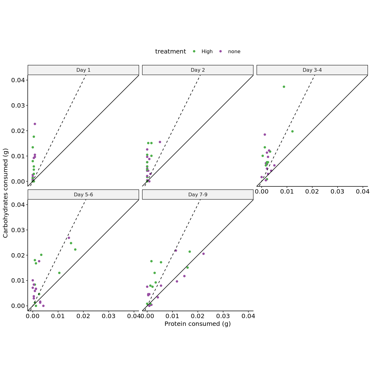
treatment_raw_plot <- dat3 |>
    ggplot(aes(x=total_p,y=total_c,color=treatment)) +
        geom_point() +
        coord_equal(ratio=1) + 
        xlab("Protein consumed (g)") + 
        ylab("Carbohydrates consumed (g)") + 
        theme_pubr() +
        geom_abline(slope = 1,linetype=1) + 
        geom_abline(slope = 2,linetype=2) + 
        facet_wrap(~day_interval) + 
        scale_color_manual(values=c("#4daf4a","#984ea3")) +
        xlim(0,0.04) +
        ylim(0,0.04)

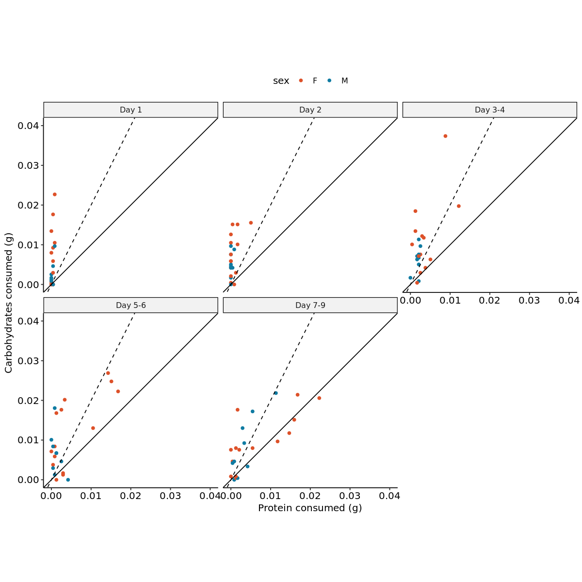
sex_raw_plot <- dat3 |>
    ggplot(aes(x=total_p,y=total_c,color=sex)) +
        geom_point() +
        coord_equal(ratio=1) + 
        xlab("Protein consumed (g)") + 
        ylab("Carbohydrates consumed (g)") + 
        theme_pubr() +
        geom_abline(slope = 1,linetype=1) + 
        geom_abline(slope = 2,linetype=2) + 
        facet_wrap(~day_interval) + 
        scale_color_manual(values=c("#dd5129","#0f7ba2")) +
        xlim(0,0.04) +
        ylim(0,0.04)

treatment raw plot

In [15]:

treatment_raw_plot

sex raw plot

In [16]:

sex_raw_plot

save plots to disk

In [17]:

# Define the output directory
output_dir <- here('output/field_cage_experiment/raw_visualization/')

# List of plots and their corresponding file names
plots <- list(
  "intake_target_treatment_raw_graph" = treatment_raw_plot,
  "intake_target_sex_raw_graph" = sex_raw_plot
)

# Loop through each plot and save it
for (name in names(plots)) {
  ggsave(
    filename = file.path(output_dir, paste0(name, ".png")),
    plot = plots[[name]],
    width = 15, height = 10, dpi = 300
  )
}

Modeling

Model Comparison Overview: Locust Nutrient Consumption

This analysis focuses on the nutrient cimulative consumption of carbohydrates (cumulative_total_c) and proteins (cumulative_total_p) by locusts over time (interval), with key predictors such as sex, treatment, and other covariates. The following six Generalized Additive Models (GAMs) are used to assess the impact of these factors:

Model 1: Full Model with Random Effects for Repeated Measures

mod1 <- gam(list( 
  cumulative_total_c ~ sex + interval + treatment + s(id, bs="re"),  
  cumulative_total_p ~ sex + interval + treatment + s(id, bs="re")),
  family=mvn(d=2), select=TRUE, data=dat3
)

Fixed Effects: Includes sex, interval, and treatment.
Random Effects:
- s(id, bs="re"): Random effect to account for repeated measures on individual locusts (id), but note the sample size may not be sufficient for this structure.
Purpose: This model captures the effects of sex, time, and treatment while accounting for individual locust variability.

Model 2: Interaction Between Interval and Treatment, No Smooth Terms

mod2 <- gam(list( 
  cumulative_total_c ~ sex + (interval) * treatment,   
  cumulative_total_p ~ sex + (interval) * treatment),
  family=mvn(d=2), select=TRUE, data=dat3
)

Fixed Effects: Includes sex, interval, treatment, and their interaction.
Purpose: Simplifies the model by removing the smooth term for initial mass, focusing solely on the interaction between time and treatment.

Model 3: Fixed Effects for Sex Only

mod3 <- gam(list( 
  cumulative_total_c ~ sex,
  cumulative_otal_p ~ sex),
  family=mvn(d=2), select=TRUE, data=dat3
)

Fixed Effects: Only includes sex.
Purpose: This model isolates the effect of sex on nutrient consumption without considering time, treatment, or mass.

Model 4: Fixed Effects for Treatment Only

mod4 <- gam(list( 
  cumulative_total_c ~ treatment,
  cumulative_total_p ~ treatment),
  family=mvn(d=2), select=TRUE, data=dat3
)

Fixed Effects: Only includes treatment.
Purpose: This model tests the direct effect of treatment on nutrient consumption without accounting for sex, time, or mass.

Model 5: Intercept-Only Model (Null Model)

mod5 <- gam(list( 
  cumulative_total_c ~ 1,
  cumulative_total_p ~ 1),
  family=mvn(d=2), select=TRUE, data=dat3
)

Fixed Effects: Only includes an intercept term.
Purpose: Serves as a null model, estimating the overall mean of carbohydrate and protein consumption without considering any predictors.

Summary

By comparing these models, we can assess the influence of sex, treatment, interval, and initial mass on locust nutrient consumption. The models range from full random effects models (Model 1) to simplified intercept-only models (Model 6), allowing for a thorough exploration of the factors driving nutrient consumption.

In [18]:


mod1 <- gam(list( 
  cumulative_total_c ~  sex  +  interval + treatment + s(id, bs="re"), 
  cumulative_total_p ~  sex + interval + treatment  + s(id, bs="re")),
  family=mvn(d=2),select=TRUE, data=dat3
)


mod2 <- gam(list( 
  cumulative_total_c ~  sex + interval * treatment,   
  cumulative_total_p ~  sex + interval * treatment),
  family=mvn(d=2),select=TRUE, data=dat3
)

mod3 <- gam(list( 
  cumulative_total_c ~  sex ,
  cumulative_total_p ~  sex),
  family=mvn(d=2),select=TRUE, data=dat3
)

mod4 <- gam(list( 
  cumulative_total_c ~   treatment,
  cumulative_total_p ~   treatment),
  family=mvn(d=2),select=TRUE, data=dat3
)

mod5 <- gam(list( 
  cumulative_total_c ~   1,
  cumulative_total_p ~   1),
  family=mvn(d=2),select=TRUE, data=dat3
)

Model Diagnostics

In [19]:

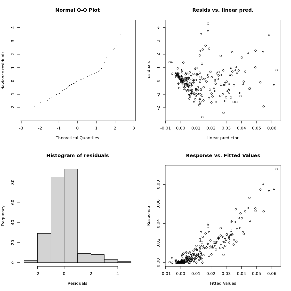
gam.check(mod1)


Method: REML   Optimizer: outer newton
full convergence after 6 iterations.
Gradient range [-0.000203556,0.0005737438]
(score -954.8838 & scale 1).
Hessian positive definite, eigenvalue range [1.80807,7.847553].
Model rank =  63 / 63 

Basis dimension (k) checking results. Low p-value (k-index<1) may
indicate that k is too low, especially if edf is close to k'.

          k'  edf k-index p-value
s(id)   23.0 17.6      NA      NA
s.1(id) 23.0 10.6      NA      NA

These diagnostic plots indicate these models could be improved. I think for descriptive uses these models are okay.

Assuming a gaussian distribution is probably limiting here.

Model selection criteria

In [20]:

# Model selection using AIC, BIC, and AICc
bic <- BIC(mod1, mod2, mod3, mod4, mod5) |>  # Bayesian Information Criterion
    mutate(deltaBIC = BIC - min(BIC)) |>
    rownames_to_column('model') |>
    dplyr::select(model,BIC,deltaBIC)

aic <- AIC(mod1, mod2, mod3, mod4, mod5)  |>  # Akaike Information Criterion
    mutate(deltaAIC = AIC - min(AIC)) |>
    rownames_to_column('model') |>
    dplyr::select(model,AIC,deltaAIC)

aicc <- AICc(mod1, mod2, mod3, mod4, mod5)  |>  # AIC adjusted for small sample size
    mutate(deltaAICc = AICc - min(AICc)) |>
    rownames_to_column('model') |>
    dplyr::select(model,AICc,deltaAICc)

model_selection_tables <- bic |>
    left_join(aic,by='model') |>
    left_join(aicc,by='model') |>
    mutate(experiment = 'locust_intake_target_through_time')

In [21]:

model_selection_tables |> arrange(deltaAIC)

A data.frame: 5 × 8
model	BIC	deltaBIC	AIC	deltaAIC	AICc	deltaAICc	experiment
<chr>	<dbl>	<dbl>	<dbl>	<dbl>	<dbl>	<dbl>	<chr>
mod1	-1959.594	0.00000	-2086.993	0.0000	-2021.876	0.00000	locust_intake_target_through_time
mod2	-1907.268	52.32555	-1975.891	111.1021	-1961.285	60.59134	locust_intake_target_through_time
mod3	-1900.026	59.56801	-1919.240	167.7533	-1918.193	103.68257	locust_intake_target_through_time
mod4	-1895.604	63.98977	-1914.818	172.1751	-1913.772	108.10433	locust_intake_target_through_time
mod5	-1898.807	60.78667	-1912.532	174.4619	-1911.981	109.89482	locust_intake_target_through_time

All model selection criteria agreed that mod1 was the best model

Final Model Summary

In [22]:

summary(mod1)


Family: Multivariate normal 
Link function: 

Formula:
cumulative_total_c ~ sex + interval + treatment + s(id, bs = "re")
cumulative_total_p ~ sex + interval + treatment + s(id, bs = "re")

Parametric coefficients:
                  Estimate Std. Error z value Pr(>|z|)    
(Intercept)      0.0125868  0.0036504   3.448 0.000565 ***
sexM            -0.0108931  0.0041592  -2.619 0.008818 ** 
interval2        0.0066835  0.0025232   2.649 0.008077 ** 
interval3        0.0160330  0.0025232   6.354 2.09e-10 ***
interval4        0.0259670  0.0025232  10.291  < 2e-16 ***
interval5        0.0350061  0.0025232  13.874  < 2e-16 ***
treatmentnone   -0.0061015  0.0040947  -1.490 0.136202    
(Intercept).1    0.0022792  0.0014613   1.560 0.118829    
sexM.1          -0.0036943  0.0014086  -2.623 0.008726 ** 
interval2.1      0.0005296  0.0014992   0.353 0.723909    
interval3.1      0.0034148  0.0014992   2.278 0.022739 *  
interval4.1      0.0071035  0.0014992   4.738 2.16e-06 ***
interval5.1      0.0125817  0.0014992   8.392  < 2e-16 ***
treatmentnone.1 -0.0009902  0.0013868  -0.714 0.475224    
---
Signif. codes:  0 ‘***’ 0.001 ‘**’ 0.01 ‘*’ 0.05 ‘.’ 0.1 ‘ ’ 1

Approximate significance of smooth terms:
          edf Ref.df Chi.sq p-value    
s(id)   17.59     20  484.7  <2e-16 ***
s.1(id) 10.61     20  110.7   0.381    
---
Signif. codes:  0 ‘***’ 0.001 ‘**’ 0.01 ‘*’ 0.05 ‘.’ 0.1 ‘ ’ 1

Deviance explained = 73.4%
-REML = -954.88  Scale est. = 1         n = 115

Key Findings

Sex Effect: Males consumed significantly less protein and carbohydrates than females.
Time (Interval) Effect:
- Protein consumption increased significantly in later intervals, especially interval 5 (p < 0.001).
- Carbohydrate consumption also showed increases in later intervals, notably in intervals 3, 4, and 5.
Fertilization Treatment: Locusts in plots without nitrogen fertilization consumed less protein (p = 0.0285), but the effect was not significant for carbohydrates.
Random Effect: There was no significant individual effect (s(id)), indicating individual locusts did not contribute heavily to variation.
Deviance Explained: The model explained 20.5% of the variation in nutrient consumption.

Model outputs

I am going to get the estimated marginal means for inter,date, and treatment:date and output as a dataframe

I will write out the transformed raw data to disk

I will also write out to disk the model object

In [23]:



intake_target_exp_preds <- expand.grid(
    sex = unique(dat3$sex),
    interval = unique(dat3$interval),
    treatment = unique(dat3$treatment),
    id= unique(dat3$id)
)

# Predict carbohydrate consumption
intake_target_exp_preds$pred_carb <- predict(mod1, newdata = intake_target_exp_preds, type = "response")[, 1]

# Predict protein consumption
intake_target_exp_preds$pred_protein <- predict(mod1, newdata = intake_target_exp_preds, type = "response")[, 2]

intake_target_exp_preds

A data.frame: 460 × 6
sex	interval	treatment	id	pred_carb	pred_protein
<fct>	<fct>	<fct>	<fct>	<dbl>	<dbl>
M	1	none	1	0.005251196	0.002089128
F	1	none	1	-0.005641895	-0.001605175
M	2	none	1	0.011934674	0.002618693
F	2	none	1	0.001041583	-0.001075610
M	3	none	1	0.021284240	0.005503910
⋮	⋮	⋮	⋮	⋮	⋮
F	3	High	23	0.01278549	0.001897175
M	4	High	23	0.03361250	0.009280174
F	4	High	23	0.02271940	0.005585871
M	5	High	23	0.04265163	0.014758435
F	5	High	23	0.03175854	0.011064132

In [24]:

# Now averaging arcoss species, plot, and cage
intake_target_exp_preds2 <- intake_target_exp_preds |>
    group_by(treatment,interval) |>
    summarize(pred_carb = mean(pred_carb),
           pred_protein = mean(pred_protein))

intake_target_exp_preds2

`summarise()` has grouped output by 'treatment'. You can override using the
`.groups` argument.

A grouped_df: 10 × 4
treatment	interval	pred_carb	pred_protein
<fct>	<fct>	<dbl>	<dbl>
High	1	0.007140269	4.320264e-04
High	2	0.013823747	9.615916e-04
High	3	0.023173312	3.846809e-03
High	4	0.033107225	7.535505e-03
High	5	0.042146356	1.301377e-02
none	1	0.001038814	-5.581555e-04
none	2	0.007722292	-2.859025e-05
none	3	0.017071858	2.856627e-03
none	4	0.027005771	6.545323e-03
none	5	0.036044901	1.202358e-02

In [26]:

write.csv(intake_target_exp_preds2,here('data/processed/field_cage_experiment/intake_target_through_time_predictions.csv'),row.names=FALSE)
write.csv(dat3,here('data/processed/field_cage_experiment/intake_target_through_time_predictions_raw_data.csv'),row.names=FALSE)


write.csv(model_selection_tables, here("output/field_cage_experiment/intake_target_through_time_model_selection_criteria_results.csv"),row.names=FALSE)


# Combine the lists into a single list
models <- list('mod1'= mod1, 'mod2' = mod2, 'mod3'= mod3, 'mod4'= mod4, 'mod5'= mod5)

# Save the combined list to an RDS file
saveRDS(models, here("output/field_cage_experiment/model_objects/intake_target_through_time_models.rds"))

Section 3 - Final locust mass analysis

This model looks to see if the final mass of locusts differed between treatments.

In [27]:

locust_dat <- read_csv(here('data/raw/field_cage_experiment/LocustCageData.csv'),show_col_types = FALSE) |>
    clean_names() |>
    filter(!complete.cases(oedaleus_australis)) |>
    select(treatment,cage_num,mass_g,carb_mg_mg,protein_mg_mg,sex) |>
    drop_na() |>
    mutate(across(c(sex,cage_num),~factor(.)),
          treatment = factor(case_when(treatment == 'HighN' ~ 'high',
                                treatment == 'MedH' ~ 'medium',
                                TRUE ~ 'none'), levels= c('none','medium','high')))

New names:
• `` -> `...24`
• `` -> `...25`
• `` -> `...26`
• `` -> `...27`
• `` -> `...28`

In [28]:

locust_dat |> glimpse()

unique(locust_dat$sex)
unique(locust_dat$treatment)
unique(locust_dat$cage_num)

Rows: 292
Columns: 6
$ treatment     <fct> high, high, high, high, high, high, high, high, high, hi…
$ cage_num      <fct> 1, 1, 1, 1, 1, 1, 2, 2, 2, 2, 2, 2, 2, 2, 2, 2, 2, 2, 2,…
$ mass_g        <dbl> 0.242, 0.314, 0.288, 0.257, 0.181, 0.115, 0.132, 0.336, …
$ carb_mg_mg    <dbl> 0.1210000, 0.1210000, 0.1210000, 0.1210000, 0.1210000, 0…
$ protein_mg_mg <dbl> 0.1729659, 0.1729659, 0.1729659, 0.1729659, 0.1729659, 0…
$ sex           <fct> F, F, F, F, M, M, M, F, F, M, M, M, F, F, F, F, F, F, F,…

Levels:

high
none
medium

Levels:

'none'
'medium'
'high'

Levels:

'1'
'2'
'3'
'4'
'5'
'6'
'7'
'8'
'9'
'10'
'11'
'12'
'13'
'14'
'15'
'16'
'17'
'18'
'19'
'20'
'21'
'22'
'23'
'24'
'25'
'26'
'27'
'28'
'29'
'30'
'31'
'32'
'33'
'34'
'35'
'36'

Building model

In [29]:

mod <- gam(mass_g ~
               sex +
               treatment +
               s(carb_mg_mg,protein_mg_mg) +
               s(cage_num,bs='re'),
        family=scat(),
        select=TRUE,
        data=locust_dat)

Model appraisal

In [30]:

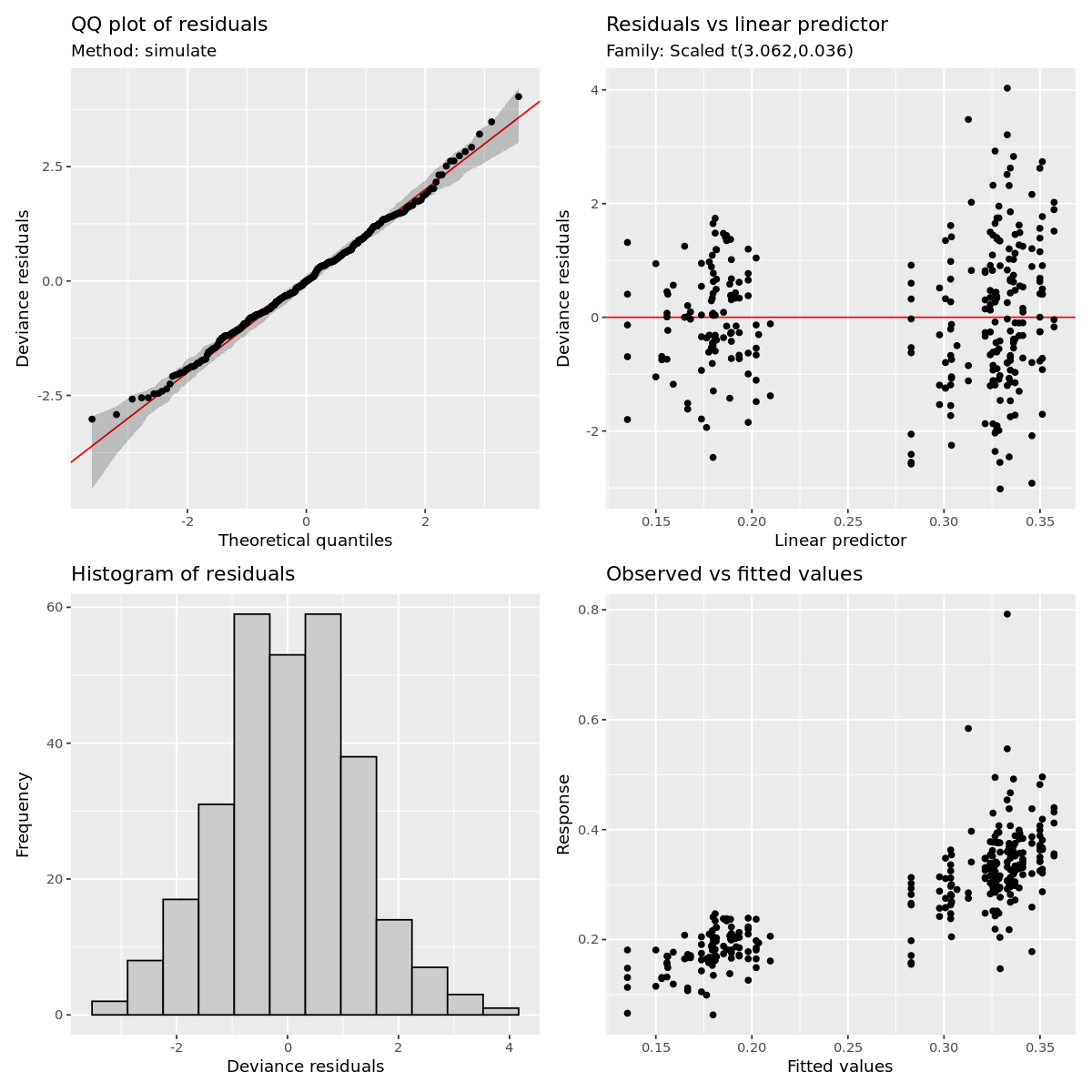
gratia::appraise(mod)

Model summary

In [31]:

summary(mod)


Family: Scaled t(3.062,0.036) 
Link function: identity 

Formula:
mass_g ~ sex + treatment + s(carb_mg_mg, protein_mg_mg) + s(cage_num, 
    bs = "re")

Parametric coefficients:
                 Estimate Std. Error z value Pr(>|z|)    
(Intercept)      0.326188   0.007210  45.243   <2e-16 ***
sexM            -0.147694   0.005507 -26.820   <2e-16 ***
treatmentmedium  0.014935   0.009518   1.569    0.117    
treatmenthigh   -0.011055   0.010095  -1.095    0.273    
---
Signif. codes:  0 ‘***’ 0.001 ‘**’ 0.01 ‘*’ 0.05 ‘.’ 0.1 ‘ ’ 1

Approximate significance of smooth terms:
                                  edf Ref.df Chi.sq  p-value    
s(carb_mg_mg,protein_mg_mg)  0.001665     29  0.002    0.416    
s(cage_num)                 17.399299     33 42.160 1.78e-05 ***
---
Signif. codes:  0 ‘***’ 0.001 ‘**’ 0.01 ‘*’ 0.05 ‘.’ 0.1 ‘ ’ 1

R-sq.(adj) =  0.617   Deviance explained = 61.6%
-REML = -427.13  Scale est. = 1         n = 292

Key Findings

Sex Effect: Males are significantly lighter than females (p < 0.001).
Fertilization Treatment:
- No significant effect of medium or high fertilization treatments on locust mass (p > 0.1).
Nutrient Content: The interaction between carbohydrate and protein content did not significantly affect locust mass (p = 0.416).
Cage Effect: Significant variability in mass was attributed to differences between cages (p = 1.78e-05).
Deviance Explained: The model explains 61.6% of the variance in locust mass.

Model outputs

I dont need the estimated marginal means since there was no difference. I will just save the model to disk?

In [32]:

saveRDS(mod, here("output/field_cage_experiment/model_objects/final_locust_weight_by_field_cage_treatment_models.rds"))

2-2 cage - locust physiology anaylses

Field cage nutrient analysis – Locust Physiology

Section 1 - analyze locust weight, surivial, and # adult in field cages

read in data

Now create two dataframes

save to disk for figure construction

Section 2 - analyze locust nutrient rebalancing through time

read in data

data management step 1

data management step 2

raw data visualization

treatment raw plot

sex raw plot

save plots to disk

Modeling

Model Comparison Overview: Locust Nutrient Consumption

Model 1: Full Model with Random Effects for Repeated Measures

Model 2: Interaction Between Interval and Treatment, No Smooth Terms

Model 3: Fixed Effects for Sex Only

Model 4: Fixed Effects for Treatment Only

Model 5: Intercept-Only Model (Null Model)

Summary

Model Diagnostics

Model selection criteria

Final Model Summary

Key Findings

Model outputs

Section 3 - Final locust mass analysis

Building model

Model appraisal

Model summary

Key Findings

Model outputs