This section covers the spatial modeling for australian plague locusts

section 1: data management
section 2: outbreak modeling
section 3: nil-observatiom modeling
section 4: outbreak and mean annual preciptation modeling

We will do basic modeling and saving relevant data to disk

Another notebook later in the series will create mansucript figures and tables

Section 1 - Data management

In [89]:

load_packages <- function(packages) {
  # Check for uninstalled packages
  uninstalled <- packages[!packages %in% installed.packages()[,"Package"]]
  
  # Install uninstalled packages
  if(length(uninstalled)) install.packages(uninstalled, dependencies = TRUE)

  # Load all packages
  for (pkg in packages) {
    if (!require(pkg, character.only = TRUE, quietly = TRUE)) {
      message(paste("Failed to load package:", pkg))
    }
  }
}

# List of packages to check, install, and load
packages <- c("mgcv", "gratia", "sf","rnaturalearth",
              "ggpubr", "patchwork", "broom", "knitr", "janitor", 
              "here","ggpubr","MetBrewer","GGally","tidyverse")

load_packages(packages)

i_am('README.md')


# Setting R options for jupyterlab
options(repr.plot.width = 10, repr.plot.height = 10,repr.matrix.max.rows=10)

here() starts at /home/datascience/herbivore_nutrient_interactions

read in data

filter species for APL
manage data into long format
select variables used for modeling
create outbreak and nil observation datasets

In [90]:

apl_dat <- read_csv(here('data/processed/spatial_modeling/apl_survey_remote_sense_data.csv'),show_col_types = FALSE)

In [32]:

apl_locust_dat <- apl_dat |>
    clean_names() |>
  mutate(adult_density = str_remove_all(adult_density, "[{}]"),
         nymph_density = str_remove_all(nymph_density, "[{}]")) %>%
  separate_rows(adult_density, sep = ", ") %>%
  separate(adult_density, into = c("adult_density", "adult_density_count"), sep = ": ") %>%
  separate_rows(nymph_density, sep = ", ") %>%
  separate(nymph_density, into = c("nymph_density", "nymph_density_count"), sep = ": ") %>%
  mutate(across(c(adult_density, adult_density_count, nymph_density, nymph_density_count), as.numeric)) |> 
  distinct() |>
  group_by(polygon_id,species) |>
  mutate(total_observations = n())

In [4]:

unique(apl_locust_dat$ecoregion)

'Great Victoria desert'
'Central Ranges xeric scrub'
'Tirari-Sturt stony desert'
'Simpson desert'
'Great Sandy-Tanami desert'
'Mitchell Grass Downs'
'Carpentaria tropical savanna'
'Flinders-Lofty montane woodlands'
'Murray-Darling woodlands and mallee'
'Southeast Australia temperate savanna'
'Naracoorte woodlands'
'Southeast Australia temperate forests'
'Eastern Australia mulga shrublands'
'Brigalow tropical savanna'
'Eastern Australian temperate forests'
'Eyre and York mallee'

In [33]:

names(apl_locust_dat)

'unnamed_0'
'species'
'polygon_id'
'date'
'longitude'
'latitude'
'data_quality'
'nymph_density'
'nymph_density_count'
'adult_density'
'adult_density_count'
'data_quality_total_count'
'adult_density_total_count'
'nymph_density_total_count'
'geometry_x'
'x0_bdod_median'
'x10_silt_median'
'x1_cec_median'
'x2_cfvo_median'
'x3_clay_median'
'x4_nitrogen_median'
'x5_ocd_median'
'x6_ocs_single_band'
'x7_phh2o_median'
'x8_sand_median'
'x9_soc_median'
'awc_awc_000_005_ev'
'awc_awc_005_015_ev'
'bdw_bdw_000_005_ev'
'bdw_bdw_005_015_ev'
'cly_cly_000_005_ev'
'cly_cly_005_015_ev'
'ece_ece_000_005_ev'
'ece_ece_005_015_ev'
'nto_nto_000_005_ev'
'nto_nto_005_015_ev'
'pto_pto_000_005_ev'
'pto_pto_005_015_ev'
'slt_slt_000_005_ev'
'slt_slt_005_015_ev'
'snd_snd_000_005_ev'
'snd_snd_005_015_ev'
'soc_soc_000_005_ev'
'soc_soc_005_015_ev'
'bio01'
'bio02'
'bio03'
'bio04'
'bio05'
'bio06'
'bio07'
'bio08'
'bio09'
'bio10'
'bio11'
'bio12'
'bio13'
'bio14'
'bio15'
'bio16'
'bio17'
'bio18'
'bio19'
'elevation'
'p_hc_p_hc_000_005_ev'
'p_hc_p_hc_005_015_ev'
'tree_canopy_cover'
'ecoregion'
'geometry_y'
'total_observations'

In [35]:

apl_outbreak_dat <- apl_locust_dat |>
    ungroup() |>
    filter(species == 11 & nymph_density == 4) |>
    select(polygon_id,longitude,latitude,nymph_density,nymph_density_count,nymph_density_total_count,
           nto_nto_000_005_ev,nto_nto_005_015_ev,pto_pto_005_015_ev,pto_pto_000_005_ev,ecoregion,bio12) |>
    group_by(polygon_id) |>
    mutate(nitrogen = sum(nto_nto_005_015_ev,nto_nto_000_005_ev)/2, 
           phosphorus = sum(pto_pto_005_015_ev,pto_pto_000_005_ev)/2,
          ecoregion = factor(ecoregion)) |>
    select(!c(nto_nto_000_005_ev,nto_nto_005_015_ev,pto_pto_005_015_ev,pto_pto_000_005_ev))  |>
    distinct()

apl_nil_dat <- apl_locust_dat |>
    ungroup() |>
    filter(species == 11 & nymph_density == 0) |>
    select(polygon_id,longitude,latitude,nymph_density,nymph_density_count,nymph_density_total_count,
           nto_nto_000_005_ev,nto_nto_005_015_ev,pto_pto_005_015_ev,pto_pto_000_005_ev,ecoregion,bio12) |>
    group_by(polygon_id) |>
    mutate(nitrogen = sum(nto_nto_005_015_ev,nto_nto_000_005_ev)/2, 
           phosphorus = sum(pto_pto_005_015_ev,pto_pto_000_005_ev)/2,
          ecoregion = factor(ecoregion)) |>
    select(!c(nto_nto_000_005_ev,nto_nto_005_015_ev,pto_pto_005_015_ev,pto_pto_000_005_ev)) |>
    distinct()

save to disk for further use

In [36]:


write.csv(apl_outbreak_dat,here('data/processed/spatial_modeling/spatial_modeling_locust_outbreak_model_data.csv'),row.names=FALSE)

write.csv(apl_nil_dat,here('data/processed/spatial_modeling/spatial_modeling_locust_nil_model_data.csv'),row.names=FALSE)

Section 2 - outbreak modeling

In [48]:

outbreak_data <- read_csv(here('data/processed/spatial_modeling/spatial_modeling_locust_outbreak_model_data.csv'),
                          show_col_types = FALSE) |>
    mutate(ecoregion = factor(ecoregion),nymph_density_count=as.integer(nymph_density_count)) |>
    #Filtering out extreme values
    filter(nymph_density_count <= 50 & nitrogen <= 0.4)  |>
    drop_na()

Raw data visualization

In [49]:

head(outbreak_data,1)
nrow(outbreak_data)

A tibble: 1 × 10
polygon_id	longitude	latitude	nymph_density	nymph_density_count	nymph_density_total_count	ecoregion	bio12	nitrogen	phosphorus
<dbl>	<dbl>	<dbl>	<dbl>	<int>	<dbl>	<fct>	<dbl>	<dbl>	<dbl>
162921	137.1195	-33.36002	4	1	1	Eyre and York mallee	331	0.07035461	0.02197414

6618

In [50]:

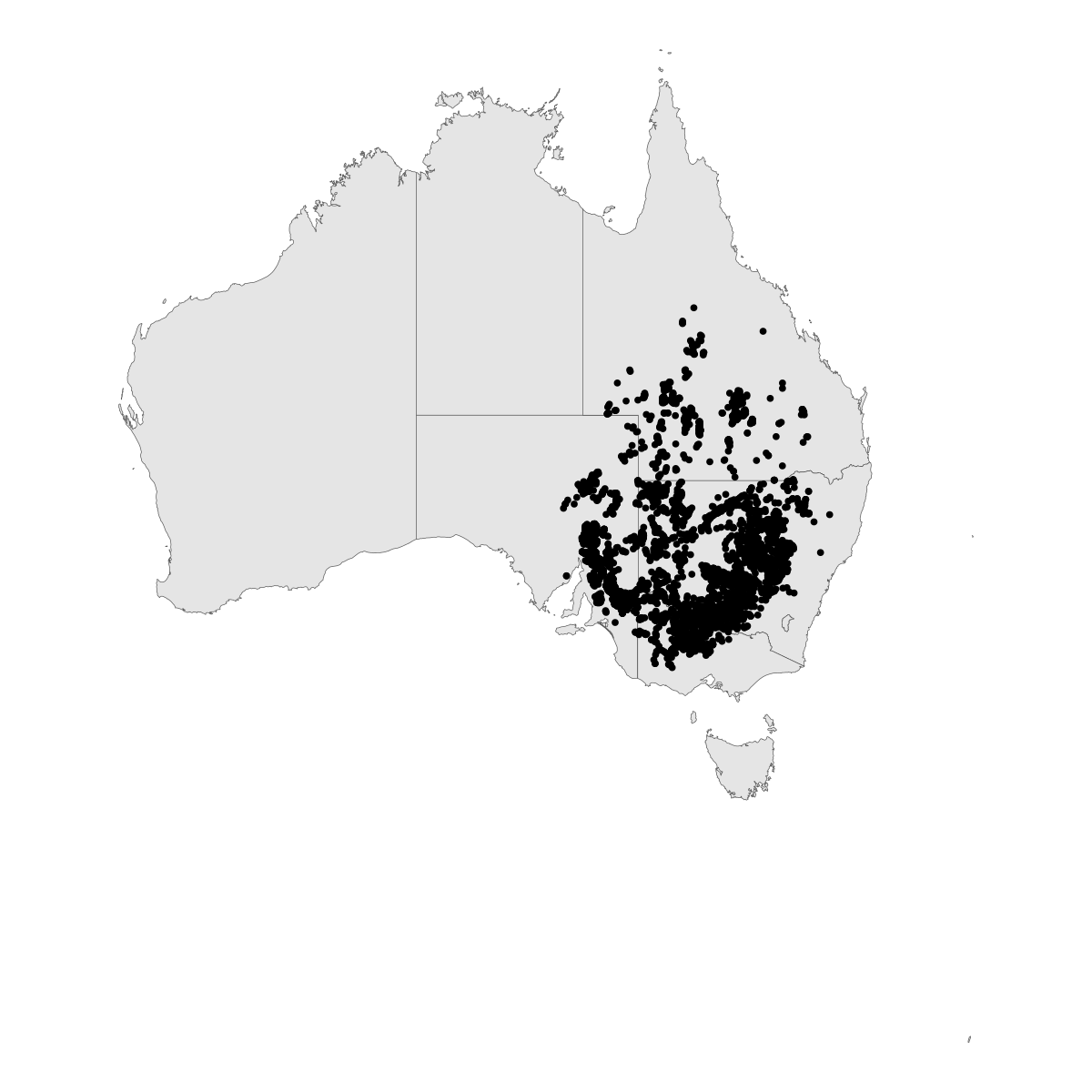
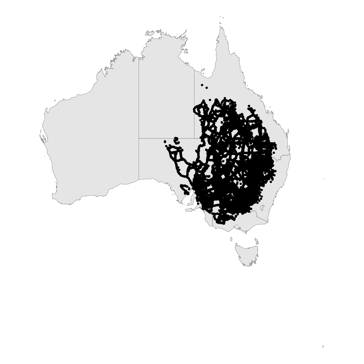
aus <- ne_states(country = 'Australia')


map_dat <- outbreak_data |>
    select(polygon_id,latitude,longitude,nymph_density_count) |>
    st_as_sf(coords = c('longitude','latitude'),
                   crs= "+proj=longlat +datum=WGS84 +ellps=WGS84 +towgs84=0,0,0")

outbreak_point_map <- aus |>
    ggplot() +
        geom_sf() +
        geom_sf(data=map_dat) +
        theme_void() 

outbreak_point_map

In [51]:

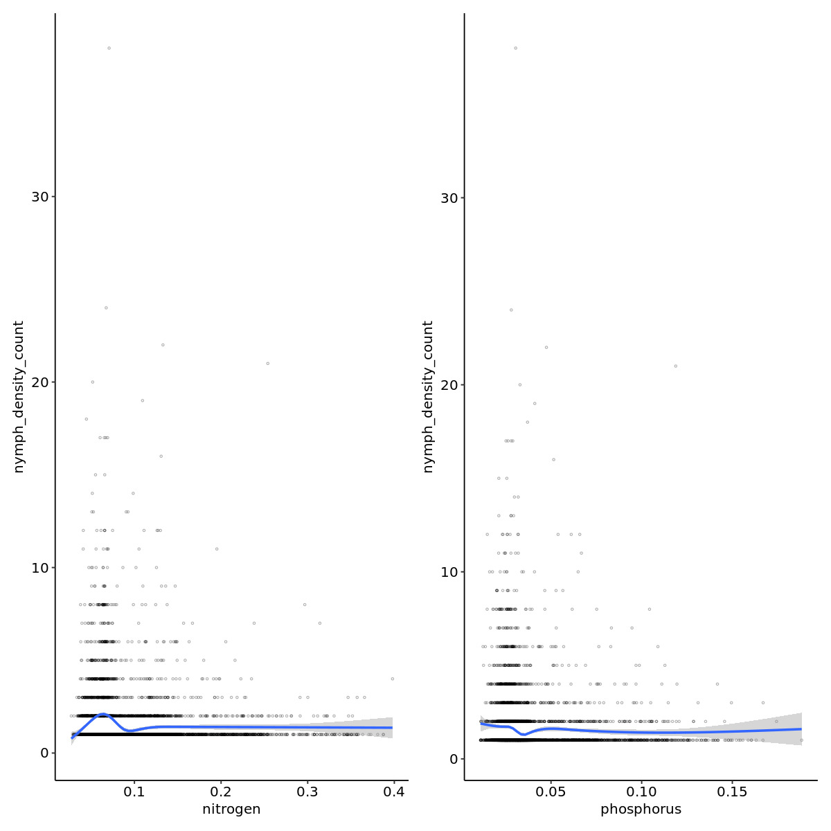
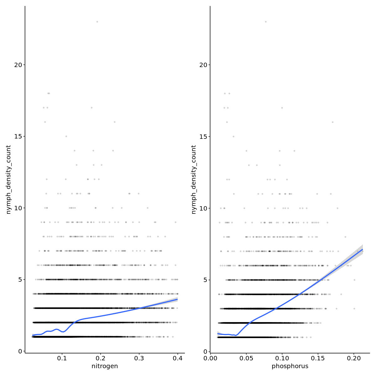
nto_plot <- outbreak_data |>
    ggplot(aes(x=nitrogen,y=nymph_density_count)) +
        geom_point(pch=21,alpha=0.3,size=0.6) +
        geom_smooth() +
        theme_pubr()

pto_plot <- outbreak_data |>
    ggplot(aes(x=phosphorus,y=nymph_density_count)) +
        geom_point(pch=21,alpha=0.3,size=0.6) +
        geom_smooth() +
        theme_pubr()

nto_plot + pto_plot

`geom_smooth()` using method = 'gam' and formula = 'y ~ s(x, bs = "cs")'
`geom_smooth()` using method = 'gam' and formula = 'y ~ s(x, bs = "cs")'

Modeling

In [11]:

summary(outbreak_data)

   polygon_id        longitude        latitude      nymph_density
 Min.   : 162921   Min.   :137.0   Min.   :-37.57   Min.   :4    
 1st Qu.: 437649   1st Qu.:139.7   1st Qu.:-34.45   1st Qu.:4    
 Median :1009080   Median :143.0   Median :-32.53   Median :4    
 Mean   : 984545   Mean   :142.9   Mean   :-32.25   Mean   :4    
 3rd Qu.:1494243   3rd Qu.:146.0   3rd Qu.:-31.04   3rd Qu.:4    
 Max.   :2092645   Max.   :151.3   Max.   :-21.08   Max.   :4    
                                                                 
 nymph_density_count nymph_density_total_count
 Min.   : 1.000      Min.   :  1.000          
 1st Qu.: 1.000      1st Qu.:  1.000          
 Median : 1.000      Median :  1.000          
 Mean   : 1.555      Mean   :  2.382          
 3rd Qu.: 1.000      3rd Qu.:  2.000          
 Max.   :38.000      Max.   :205.000          
                                              
                                 ecoregion       nitrogen      
 Southeast Australia temperate savanna:1969   Min.   :0.02707  
 Murray-Darling woodlands and mallee  :1407   1st Qu.:0.05658  
 Flinders-Lofty montane woodlands     : 954   Median :0.07917  
 Tirari-Sturt stony desert            : 584   Mean   :0.09425  
 Southeast Australia temperate forests: 508   3rd Qu.:0.11560  
 Simpson desert                       : 469   Max.   :0.61003  
 (Other)                              : 754                    
   phosphorus     
 Min.   :0.01107  
 1st Qu.:0.02562  
 Median :0.03093  
 Mean   :0.03701  
 3rd Qu.:0.03702  
 Max.   :0.23102

In [52]:

outbreak_mod <- bam(nymph_density_count ~
               s(nitrogen,k=10,bs='tp') +
               s(phosphorus,k=10,bs='tp') +
               s(nymph_density_total_count,k=25,bs='tp') +
               te(longitude,latitude,bs=c('gp','gp'),k=25) +
               s(ecoregion,bs='re'),
           select = TRUE,
           discrete = TRUE,
           nthreads = 20,
          family = tw(),
          data = outbreak_data)

Warning message in estimate.theta(theta, family, y, mu, scale = scale1, wt = G$w, :
“step failure in theta estimation”
Warning message in estimate.theta(theta, family, y, mu, scale = scale1, wt = G$w, :
“step failure in theta estimation”
Warning message in estimate.theta(theta, family, y, mu, scale = scale1, wt = G$w, :
“step failure in theta estimation”
Warning message in estimate.theta(theta, family, y, mu, scale = scale1, wt = G$w, :
“step failure in theta estimation”

In [53]:

summary(outbreak_mod)


Family: Tweedie(p=1.99) 
Link function: log 

Formula:
nymph_density_count ~ s(nitrogen, k = 10, bs = "tp") + s(phosphorus, 
    k = 10, bs = "tp") + s(nymph_density_total_count, k = 25, 
    bs = "tp") + te(longitude, latitude, bs = c("gp", "gp"), 
    k = 25) + s(ecoregion, bs = "re")

Parametric coefficients:
            Estimate Std. Error t value Pr(>|t|)    
(Intercept)  1.55154    0.03495   44.39   <2e-16 ***
---
Signif. codes:  0 ‘***’ 0.001 ‘**’ 0.01 ‘*’ 0.05 ‘.’ 0.1 ‘ ’ 1

Approximate significance of smooth terms:
                                edf Ref.df       F p-value    
s(nitrogen)                   6.273      9  25.620  <2e-16 ***
s(phosphorus)                 5.372      9  15.521  <2e-16 ***
s(nymph_density_total_count) 22.547     24 630.896  <2e-16 ***
te(longitude,latitude)       56.140    529   1.148  0.0123 *  
s(ecoregion)                  6.498     10   4.802  <2e-16 ***
---
Signif. codes:  0 ‘***’ 0.001 ‘**’ 0.01 ‘*’ 0.05 ‘.’ 0.1 ‘ ’ 1

R-sq.(adj) =  0.769   Deviance explained = 83.2%
fREML = 573.15  Scale est. = 0.064377  n = 6618

Model Diagnostics

In [54]:

k.check(outbreak_mod)

A matrix: 5 × 4 of type dbl
	k'	edf	k-index	p-value
s(nitrogen)	9	6.273422	0.9868934	0.300
s(phosphorus)	9	5.372169	1.0170037	0.955
s(nymph_density_total_count)	24	22.547306	0.9573451	0.000
te(longitude,latitude)	624	56.140461	0.8768059	0.000
s(ecoregion)	11	6.498451	NA	NA

In [55]:

concurvity(outbreak_mod,full=FALSE)

$worst

A matrix: 6 × 6 of type dbl
	para	s(nitrogen)	s(phosphorus)	s(nymph_density_total_count)	te(longitude,latitude)	s(ecoregion)
para	1.0000000	0.6883534	0.7490074	0.9880373	1.0000000	1.0000000
s(nitrogen)	0.6883534	1.0000000	0.8558808	0.7209855	0.8334426	0.7424998
s(phosphorus)	0.7490074	0.8558808	1.0000000	0.7990995	0.8208353	0.7555303
s(nymph_density_total_count)	0.9880373	0.7209855	0.7990995	1.0000000	0.9890154	0.9883096
te(longitude,latitude)	1.0000000	0.8334425	0.8208353	0.9890154	1.0000000	1.0000000
s(ecoregion)	1.0000000	0.7424998	0.7555303	0.9883096	1.0000000	1.0000000

$observed

A matrix: 6 × 6 of type dbl
	para	s(nitrogen)	s(phosphorus)	s(nymph_density_total_count)	te(longitude,latitude)	s(ecoregion)
para	1.0000000	0.5276437	0.7365579	0.9079395	0.01051500	0.01358394
s(nitrogen)	0.6883534	1.0000000	0.8458158	0.7027435	0.53716791	0.09132533
s(phosphorus)	0.7490074	0.7118931	1.0000000	0.7820410	0.03677412	0.04454272
s(nymph_density_total_count)	0.9880373	0.5505898	0.7909006	1.0000000	0.05303951	0.05005853
te(longitude,latitude)	1.0000000	0.8260141	0.7960190	0.9416384	1.00000000	0.93915689
s(ecoregion)	1.0000000	0.7322901	0.7418221	0.9249175	0.73876773	1.00000000

$estimate

A matrix: 6 × 6 of type dbl
	para	s(nitrogen)	s(phosphorus)	s(nymph_density_total_count)	te(longitude,latitude)	s(ecoregion)
para	1.0000000	0.5552027	0.6733253	0.9666292	0.006421152	0.1758807
s(nitrogen)	0.6883534	1.0000000	0.8020399	0.6832916	0.022627257	0.2610817
s(phosphorus)	0.7490074	0.7346361	1.0000000	0.7501648	0.012278002	0.1806277
s(nymph_density_total_count)	0.9880373	0.5723728	0.7178054	1.0000000	0.010464633	0.2062077
te(longitude,latitude)	1.0000000	0.7761568	0.7797759	0.9722508	1.000000000	0.9434299
s(ecoregion)	1.0000000	0.6883744	0.6950790	0.9693498	0.040977785	1.0000000

In [56]:

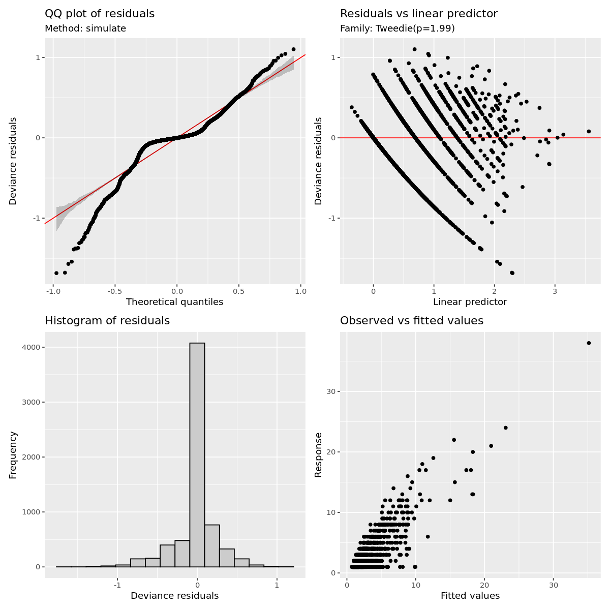
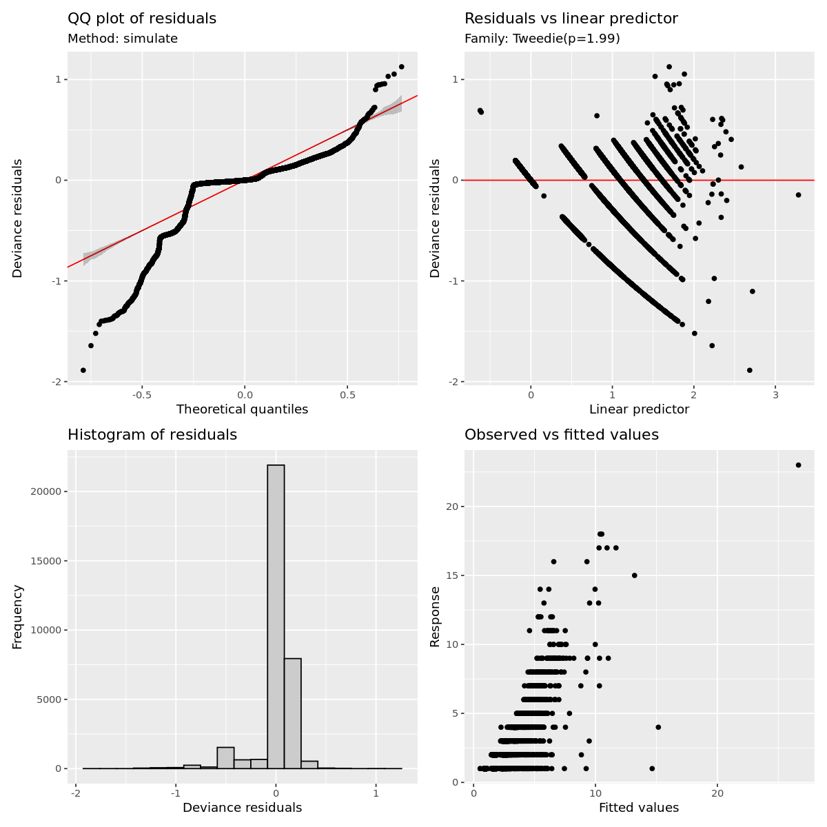
gratia::appraise(outbreak_mod)

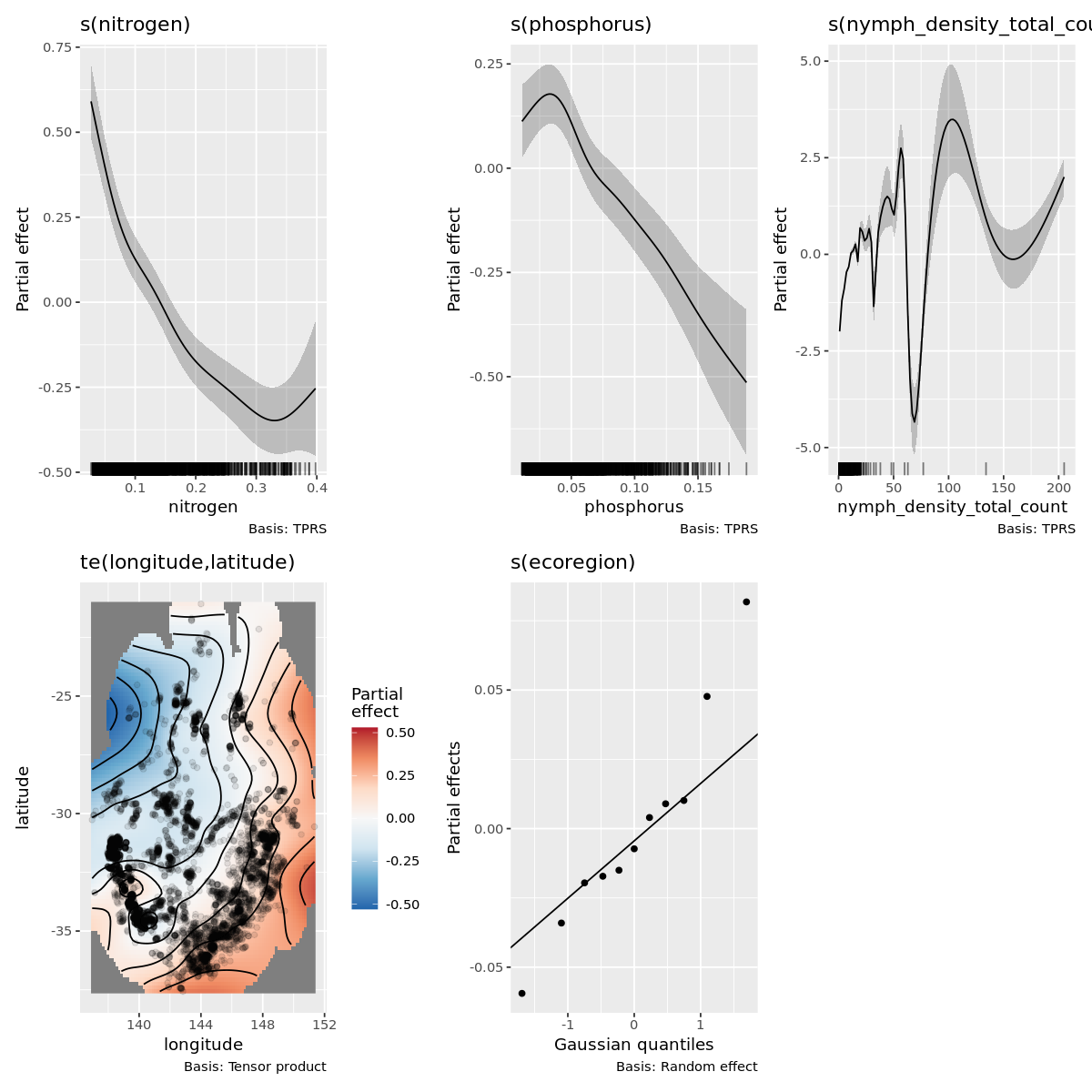
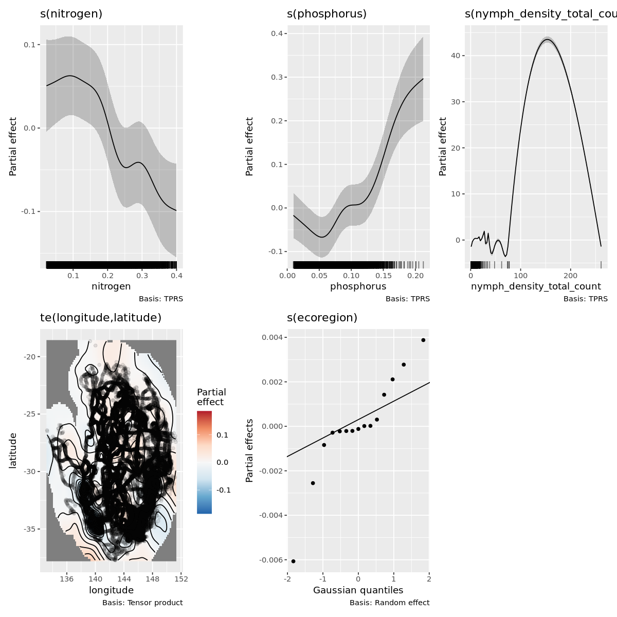
Quick model visualization

In [57]:

gratia::draw(outbreak_mod)

Outbreak modeling evaluation

Its obvious this model has some fitting issues, espicially with lower values of the dependent variable.

This is likely correlational issues between all the variable and it can muddy the interpretation as well as the number of 1 off observations.

I have already filtered out extreme grid cells that have more than 50 obersvations and that did improve the fit more.

saving outputs

In [58]:

saveRDS(outbreak_mod, here("output/spatial_modeling/model_objects/locust_outbreak_model.rds"))

In [86]:

outbreak_model_smooth_estimates <- smooth_estimates(outbreak_mod,dist=0.1)

write.csv(outbreak_model_smooth_estimates, here("output/spatial_modeling/outbreak_model_smooth_estimates.csv"),row.names=FALSE)

In [84]:

outbreak_model_smooth_estimates <- smooth_estimates(outbreak_mod,dist=0.1)

In [71]:

outbreak_model_smooth_estimates

A smooth_estimates: 10315 × 11
.smooth	.type	.by	.estimate	.se	nitrogen	phosphorus	nymph_density_total_count	longitude	latitude	ecoregion
<chr>	<chr>	<chr>	<dbl>	<dbl>	<dbl>	<dbl>	<dbl>	<dbl>	<dbl>	<fct>
s(nitrogen)	TPRS	NA	0.05056327	0.02819440	0.02262577	NA	NA	NA	NA	NA
s(nitrogen)	TPRS	NA	0.05127533	0.02774333	0.02643393	NA	NA	NA	NA	NA
s(nitrogen)	TPRS	NA	0.05198999	0.02732688	0.03024208	NA	NA	NA	NA	NA
s(nitrogen)	TPRS	NA	0.05271331	0.02694706	0.03405024	NA	NA	NA	NA	NA
s(nitrogen)	TPRS	NA	0.05345310	0.02660461	0.03785840	NA	NA	NA	NA	NA
⋮	⋮	⋮	⋮	⋮	⋮	⋮	⋮	⋮	⋮	⋮
s(ecoregion)	Random effect	NA	-0.0002120522	0.005155784	NA	NA	NA	NA	NA	Naracoorte woodlands
s(ecoregion)	Random effect	NA	-0.0002261551	0.004471238	NA	NA	NA	NA	NA	Simpson desert
s(ecoregion)	Random effect	NA	0.0014202656	0.004640904	NA	NA	NA	NA	NA	Southeast Australia temperate forests
s(ecoregion)	Random effect	NA	0.0038769919	0.003721848	NA	NA	NA	NA	NA	Southeast Australia temperate savanna
s(ecoregion)	Random effect	NA	0.0003027099	0.004446608	NA	NA	NA	NA	NA	Tirari-Sturt stony desert

section 3: nil-observatiom modeling

In [60]:

nil_data <- read_csv(here('data/processed/spatial_modeling/spatial_modeling_locust_nil_model_data.csv'),
                          show_col_types = FALSE)  |>
    mutate(ecoregion = factor(ecoregion),nymph_density_count=as.integer(nymph_density_count)) |>
    #Filtering out extreme values
    filter(nymph_density_count <= 50 & nitrogen <= 0.4)  |>
    drop_na()

nil_data

A tibble: 33821 × 10
polygon_id	longitude	latitude	nymph_density	nymph_density_count	nymph_density_total_count	ecoregion	bio12	nitrogen	phosphorus
<dbl>	<dbl>	<dbl>	<dbl>	<int>	<dbl>	<fct>	<dbl>	<dbl>	<dbl>
7280	133.4553	-27.06065	0	1	1	Central Ranges xeric scrub	208	0.03300749	0.02376515
8026	133.2392	-26.40242	0	1	1	Central Ranges xeric scrub	225	0.03097755	0.01831567
8097	133.2565	-26.49929	0	1	1	Central Ranges xeric scrub	223	0.03094262	0.01980745
13279	133.7368	-27.45913	0	1	1	Great Victoria desert	190	0.03268851	0.02072279
13512	133.8018	-27.53024	0	2	2	Tirari-Sturt stony desert	191	0.03296471	0.01975296
⋮	⋮	⋮	⋮	⋮	⋮	⋮	⋮	⋮	⋮
2099638	151.0890	-27.07120	0	1	1	Brigalow tropical savanna	647	0.1090968	0.05359124
2100024	151.1908	-27.21150	0	1	1	Brigalow tropical savanna	650	0.1135198	0.06566815
2100282	151.2569	-27.43300	0	1	1	Brigalow tropical savanna	628	0.1068338	0.06458026
2101656	151.1922	-26.90387	0	1	1	Brigalow tropical savanna	637	0.1206505	0.07311647
2102441	150.9997	-26.65369	0	1	1	Brigalow tropical savanna	627	0.1157181	0.03929814

Raw data visualization

In [61]:

aus <- ne_states(country = 'Australia')


map_dat <- nil_data |>
    select(polygon_id,latitude,longitude,nymph_density_count) |>
    st_as_sf(coords = c('longitude','latitude'),
                   crs= "+proj=longlat +datum=WGS84 +ellps=WGS84 +towgs84=0,0,0")

nil_point_map <- aus |>
    ggplot() +
        geom_sf() +
        geom_sf(data=map_dat) +
        theme_void() 

nil_point_map

In [62]:

nto_plot <- nil_data |>
    ggplot(aes(x=nitrogen,y=nymph_density_count)) +
        geom_point(pch=21,alpha=0.3,size=0.6) +
        geom_smooth() +
        theme_pubr()

pto_plot <- nil_data |>
    ggplot(aes(x=phosphorus,y=nymph_density_count)) +
        geom_point(pch=21,alpha=0.3,size=0.6) +
        geom_smooth() +
        theme_pubr()

nto_plot + pto_plot

`geom_smooth()` using method = 'gam' and formula = 'y ~ s(x, bs = "cs")'
`geom_smooth()` using method = 'gam' and formula = 'y ~ s(x, bs = "cs")'

Modeling

In [63]:

nil_mod <- bam(nymph_density_count ~
               s(nitrogen,k=10,bs='tp') +
               s(phosphorus,k=10,bs='tp') +
               s(nymph_density_total_count,k=25,bs='tp') +
               te(longitude,latitude,bs=c('gp','gp'),k=25) +
               s(ecoregion,bs='re'),
           select = TRUE,
           discrete = TRUE,
           nthreads = 20,
          family = tw(),
          data = nil_data)

Warning message in estimate.theta(theta, family, y, mu, scale = scale1, wt = G$w, :
“step failure in theta estimation”

Model diagnostics

In [64]:

k.check(nil_mod)

A matrix: 5 × 4 of type dbl
	k'	edf	k-index	p-value
s(nitrogen)	9	6.426332	0.9719328	0.0425
s(phosphorus)	9	6.406880	0.9658401	0.0150
s(nymph_density_total_count)	24	22.408362	0.9912682	0.3475
te(longitude,latitude)	624	131.476046	0.9515954	0.0050
s(ecoregion)	15	2.726108	NA	NA

In [65]:

concurvity(nil_mod,full=FALSE)

$worst

A matrix: 6 × 6 of type dbl
	para	s(nitrogen)	s(phosphorus)	s(nymph_density_total_count)	te(longitude,latitude)	s(ecoregion)
para	1.0000000	0.8307967	0.8685621	0.9974470	1.0000000	1.0000000
s(nitrogen)	0.8307967	1.0000000	0.9004807	0.8637565	0.8800706	0.8556794
s(phosphorus)	0.8685621	0.9004807	1.0000000	0.9113526	0.8792777	0.8697074
s(nymph_density_total_count)	0.9974470	0.8637565	0.9113526	1.0000000	0.9975198	0.9974679
te(longitude,latitude)	1.0000000	0.8800708	0.8792781	0.9975198	1.0000000	1.0000000
s(ecoregion)	1.0000000	0.8556794	0.8697074	0.9974679	1.0000000	1.0000000

$observed

A matrix: 6 × 6 of type dbl
	para	s(nitrogen)	s(phosphorus)	s(nymph_density_total_count)	te(longitude,latitude)	s(ecoregion)
para	1.0000000	0.7868098	0.8083066	0.8551952	0.004546396	0.06430443
s(nitrogen)	0.8307967	1.0000000	0.8181989	0.8397272	0.044026705	0.14027235
s(phosphorus)	0.8685621	0.8614793	1.0000000	0.9002601	0.061211576	0.17528098
s(nymph_density_total_count)	0.9974470	0.8241006	0.8383076	1.0000000	0.026668080	0.07966450
te(longitude,latitude)	1.0000000	0.8215499	0.8199754	0.8727459	1.000000000	0.81144707
s(ecoregion)	1.0000000	0.8028665	0.8106659	0.8580396	0.381904995	1.00000000

$estimate

A matrix: 6 × 6 of type dbl
	para	s(nitrogen)	s(phosphorus)	s(nymph_density_total_count)	te(longitude,latitude)	s(ecoregion)
para	1.0000000	0.6918896	0.7004913	0.9870538	0.002128188	0.1470001
s(nitrogen)	0.8307967	1.0000000	0.8371775	0.8351752	0.008066931	0.2057451
s(phosphorus)	0.8685621	0.8295907	1.0000000	0.8755378	0.003650041	0.1498173
s(nymph_density_total_count)	0.9974470	0.7624890	0.8394230	1.0000000	0.003104366	0.1504301
te(longitude,latitude)	1.0000000	0.8375298	0.7564592	0.9879833	1.000000000	0.8873811
s(ecoregion)	1.0000000	0.7927771	0.7150555	0.9872542	0.021132004	1.0000000

In [66]:

gratia::appraise(nil_mod)

In [67]:

summary(nil_mod)


Family: Tweedie(p=1.99) 
Link function: log 

Formula:
nymph_density_count ~ s(nitrogen, k = 10, bs = "tp") + s(phosphorus, 
    k = 10, bs = "tp") + s(nymph_density_total_count, k = 25, 
    bs = "tp") + te(longitude, latitude, bs = c("gp", "gp"), 
    k = 25) + s(ecoregion, bs = "re")

Parametric coefficients:
            Estimate Std. Error t value Pr(>|t|)    
(Intercept)  1.43919    0.02338   61.55   <2e-16 ***
---
Signif. codes:  0 ‘***’ 0.001 ‘**’ 0.01 ‘*’ 0.05 ‘.’ 0.1 ‘ ’ 1

Approximate significance of smooth terms:
                                 edf Ref.df        F p-value    
s(nitrogen)                    6.426      9   35.340  <2e-16 ***
s(phosphorus)                  6.407      9   28.867  <2e-16 ***
s(nymph_density_total_count)  22.408     24 3199.357  <2e-16 ***
te(longitude,latitude)       131.476    557    3.302  <2e-16 ***
s(ecoregion)                   2.726     14    0.361  0.0352 *  
---
Signif. codes:  0 ‘***’ 0.001 ‘**’ 0.01 ‘*’ 0.05 ‘.’ 0.1 ‘ ’ 1

R-sq.(adj) =  0.787   Deviance explained = 87.9%
fREML = -8209.3  Scale est. = 0.035064  n = 33821

Quick modeling visualization

In [68]:

gratia::draw(nil_mod)

saving outputs

In [69]:

saveRDS(nil_mod, here("output/spatial_modeling/model_objects/locust_nil_model.rds"))

In [87]:

outbreak_model_smooth_estimates <- smooth_estimates(nil_mod,dist=0.1)

write.csv(outbreak_model_smooth_estimates, here("output/spatial_modeling/nil_model_smooth_estimates.csv"),row.names=FALSE)

Section 4 - Locust outbreaks and mean annual preciptation modeling

Modeling

In [39]:


nil_data

A tibble: 33969 × 10
polygon_id	longitude	latitude	nymph_density	nymph_density_count	nymph_density_total_count	ecoregion	bio12	nitrogen	phosphorus
<dbl>	<dbl>	<dbl>	<dbl>	<int>	<dbl>	<fct>	<dbl>	<dbl>	<dbl>
7280	133.4553	-27.06065	0	1	1	Central Ranges xeric scrub	208	0.03300749	0.02376515
8026	133.2392	-26.40242	0	1	1	Central Ranges xeric scrub	225	0.03097755	0.01831567
8097	133.2565	-26.49929	0	1	1	Central Ranges xeric scrub	223	0.03094262	0.01980745
13279	133.7368	-27.45913	0	1	1	Great Victoria desert	190	0.03268851	0.02072279
13512	133.8018	-27.53024	0	2	2	Tirari-Sturt stony desert	191	0.03296471	0.01975296
⋮	⋮	⋮	⋮	⋮	⋮	⋮	⋮	⋮	⋮
2099638	151.0890	-27.07120	0	1	1	Brigalow tropical savanna	647	0.1090968	0.05359124
2100024	151.1908	-27.21150	0	1	1	Brigalow tropical savanna	650	0.1135198	0.06566815
2100282	151.2569	-27.43300	0	1	1	Brigalow tropical savanna	628	0.1068338	0.06458026
2101656	151.1922	-26.90387	0	1	1	Brigalow tropical savanna	637	0.1206505	0.07311647
2102441	150.9997	-26.65369	0	1	1	Brigalow tropical savanna	627	0.1157181	0.03929814

In [40]:

outbreak_map_mod <- bam(nymph_density_count ~
               s(bio12,bs='tp',k=10) +
               s(nymph_density_total_count,k=25,bs='tp') +
               te(longitude,latitude,bs=c('gp','gp'),k=25) +
               s(ecoregion,bs='re'),
           select = TRUE,
           discrete = TRUE,
           nthreads = 20,
          family = tw(),
          data = outbreak_data)

nil_map_mod <- bam(nymph_density_count ~
               s(bio12,bs='tp',k=10) +
               s(nymph_density_total_count,k=25,bs='tp') +
               te(longitude,latitude,bs=c('gp','gp'),k=25) +
               s(ecoregion,bs='re'),
           select = TRUE,
           discrete = TRUE,
           nthreads = 20,
          family = tw(),
          data = nil_data)

Warning message in estimate.theta(theta, family, y, mu, scale = scale1, wt = G$w, :
“step failure in theta estimation”
Warning message in estimate.theta(theta, family, y, mu, scale = scale1, wt = G$w, :
“step failure in theta estimation”
Warning message in estimate.theta(theta, family, y, mu, scale = scale1, wt = G$w, :
“step failure in theta estimation”
Warning message in estimate.theta(theta, family, y, mu, scale = scale1, wt = G$w, :
“step failure in theta estimation”

saving outputs

In [41]:

saveRDS(outbreak_map_mod, here("output/spatial_modeling/model_objects/locust_outbreak_map_model.rds"))
saveRDS(nil_map_mod, here("output/spatial_modeling/model_objects/locust_nil_map_model.rds"))

In [88]:

map_outbreak_model_smooth_estimates <- smooth_estimates(outbreak_map_mod,dist=0.1)
map_nill_model_smooth_estimates <- smooth_estimates(nil_map_mod,dist=0.1)

write.csv(map_outbreak_model_smooth_estimates, here("output/spatial_modeling/map_outbreak_model_smooth_estimates.csv"),row.names=FALSE)
write.csv(map_nill_model_smooth_estimates, here("output/spatial_modeling/map_nill_model_smooth_estimates.csv"),row.names=FALSE)

3-4 spatial modeling - modeling and data visualization

Australia Plauge Locust Modeling

Section 1 - Data management

read in data

save to disk for further use

Section 2 - outbreak modeling

Raw data visualization

Modeling

Model Diagnostics

Quick model visualization

Outbreak modeling evaluation

saving outputs

section 3: nil-observatiom modeling

Raw data visualization

Modeling

Model diagnostics

Quick modeling visualization

saving outputs

Section 4 - Locust outbreaks and mean annual preciptation modeling

Modeling

saving outputs